When you take a basic calculus course, you learn how to find where a function \(f(x)\) reaches its local minimum (or maximum) by setting its derivative \(f'(x)\) to zero. At points where the derivative is zero, the function is either a local maximum, a local minimum, or a saddle point (neither a max nor a min). We often decide which case it is by checking the second derivative or performing more extensive tests.
Once we move into multiple variables—like a function \(f(\mathbf{x})\) with \(\mathbf{x} = (x_1, x_2, \dots, x_n)\)—we use the gradient instead of a single derivative. The gradient is simply the vector of partial derivatives. You can think of it as an arrow that points along the steepest slope of the function in an \(n\)-dimensional space.
Gradient Descent is an algorithm that repeatedly tweaks the parameters \(\theta\) of your model (or function) in the direction that reduces your loss (sometimes also called cost) the most at every step. If you imagine a hilly landscape, gradient descent is like walking downhill in small steps until you (hopefully) reach a valley. The size of these steps is extremely important—if they are too large, you can end up leaping right over the valley and climbing another hill instead.
Suppose you have a function \(J(\theta)\) you want to minimize. If \(\theta\) is a single number, you use its ordinary derivative. If \(\theta\) is a vector, the concept is identical but you use a gradient. You start by picking an initial guess \(\theta^{(0)}\), then repeatedly update \(\theta\) according to:
\[ \theta^{(k+1)} = \theta^{(k)} - \alpha \nabla_\theta J(\theta^{(k)}) \]
where \(\alpha\) is called the learning rate. This learning rate decides how big your step is each time.
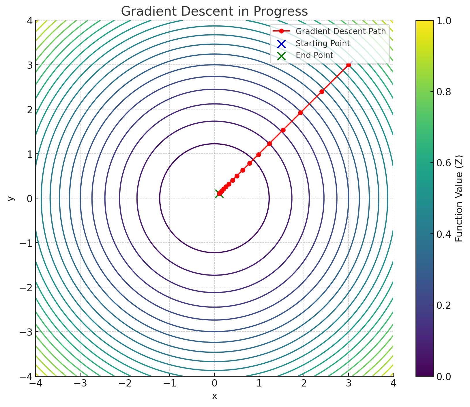
As a simple illustration, consider minimizing the function \(z = x^2 + y^2\). It’s clear that the minimum is at \((x, y) = (0, 0)\). If you start at \((3, 3)\) with a learning rate \(\alpha = 0.1\), the algorithm repeatedly steps you closer to \((0, 0)\). After about fifteen iterations, you’ll find yourself very near the origin, at \((0.106, 0.106)\), which is practically zero for many applications.
Adam (Adaptive Moment Estimation) addresses common pitfalls in “vanilla” gradient descent. These include oscillating around minima, getting stuck on saddle points, and extremely slow convergence in shallow regions of the loss surface. Adam combines two key ideas—momentum and RMSProp—into a single optimizer.
Plain gradient descent only considers the current gradient. If this gradient is noisy or misleading for just one step, your parameter update can overshoot or head in an unhelpful direction. Momentum introduces an exponentially decaying average of past gradients. Recent gradients get the most weight, older gradients still have some influence (though less so), and this “memory” of past updates helps reduce jittery behavior. Formally, the momentum term \(m_t\) is computed as:
\[ m_t = \beta_1 m_{t-1} + (1 - \beta_1) g_t \]
where \(g_t\) is the gradient at step \(t\) and \(\beta_1\) (often around 0.9) is the decay rate determining how quickly older gradient terms fade away.
At the very beginning (when \(t = 1, 2, \dots\) is still small), \(m_t\) is too small because it started at zero. To compensate, we apply a bias correction:
\[ m_t^{\text{corrected}} = \frac{m_t}{1 - \beta_1^t} \]
This scaling essentially corrects the fact that you had no “past” gradients at initialization, giving the momentum an appropriate boost so it reflects the actual average of recent gradients.
RMSProp considers not just the gradient but the square of the gradient. The reason is that if a particular parameter consistently has large gradients, you might want to dampen your updates for that parameter to avoid wild oscillations. Conversely, if the gradients for another parameter remain small, you might want to make larger adjustments. You achieve this by keeping an exponentially weighted average of the squared gradients:
\[ v_t = \beta_2 v_{t-1} + (1 - \beta_2) g_t^2 \]
where \(\beta_2\) is another decay factor, often set around 0.999, and \(v_t\) accumulates the history of squared gradients.
Similar to \(m_t\), the value of \(v_t\) will be artificially small when \(t\) is small because of the zero initialization. So we correct it with:
\[ v_t^{\text{corrected}} = \frac{v_t}{1 - \beta_2^t} \]
This ensures that \(v_t\) isn’t stuck at lower values just because the optimizer started at zero.
Adam uses both momentum (\(m_t\)) and this RMSProp-like term (\(v_t\)) to update your parameters. The update rule for \(\theta_t\) is:
\[ \theta_t = \theta_{t-1} - \frac{\alpha}{\sqrt{v_t^{\text{corrected}}} + \epsilon} m_t^{\text{corrected}} \]
where \(\alpha\) is the base learning rate, \(m_t^{\text{corrected}}\) is the bias-corrected momentum term, \(v_t^{\text{corrected}}\) is the bias-corrected squared-gradient term, and \(\epsilon\) (often \(10^{-8}\)) is a small constant to avoid dividing by zero. The division by \(\sqrt{v_t^{\text{corrected}}} + \epsilon\) effectively gives each parameter \(\theta_i\) its own adaptive learning rate based on the recent history of its gradients.
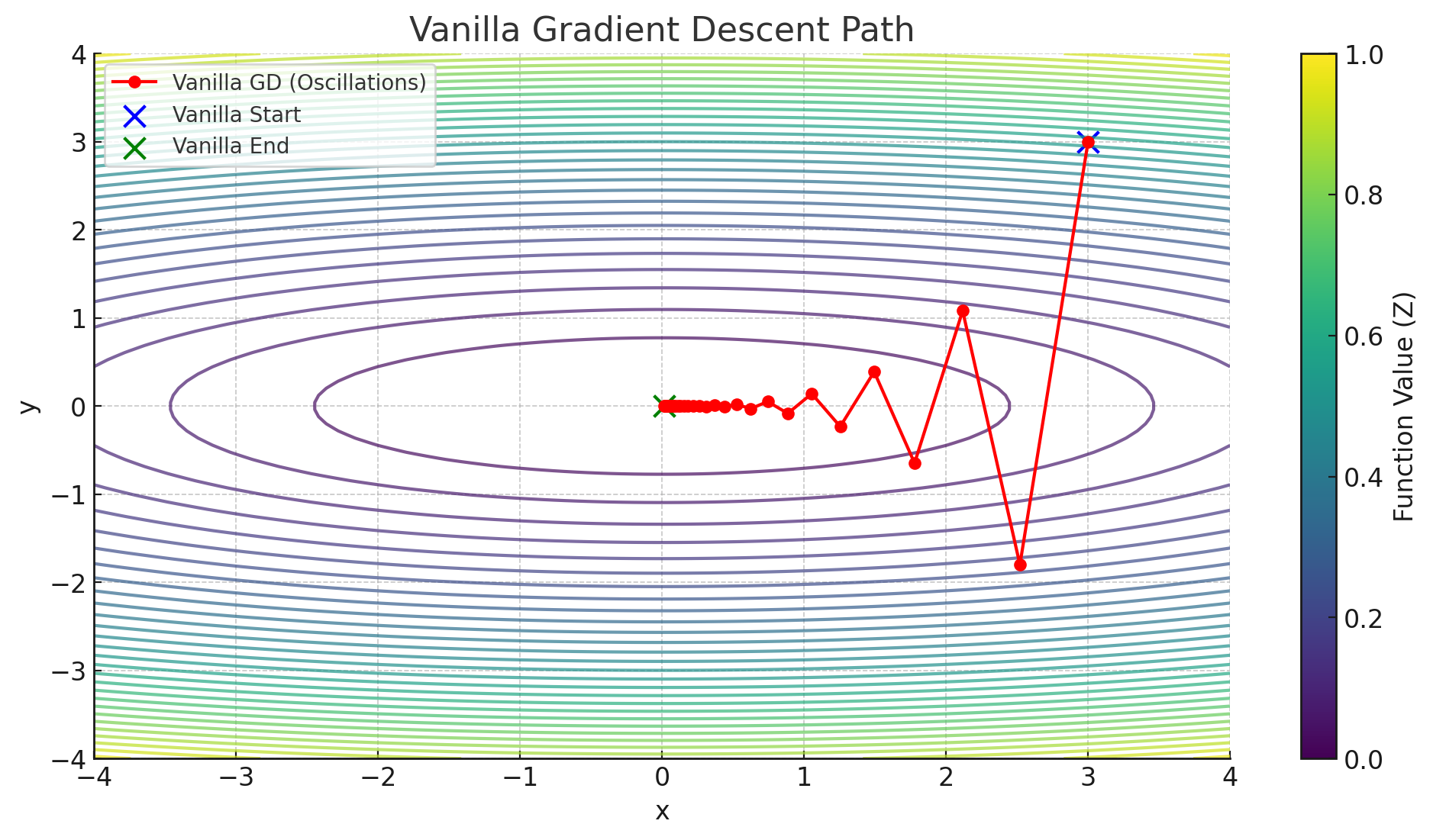
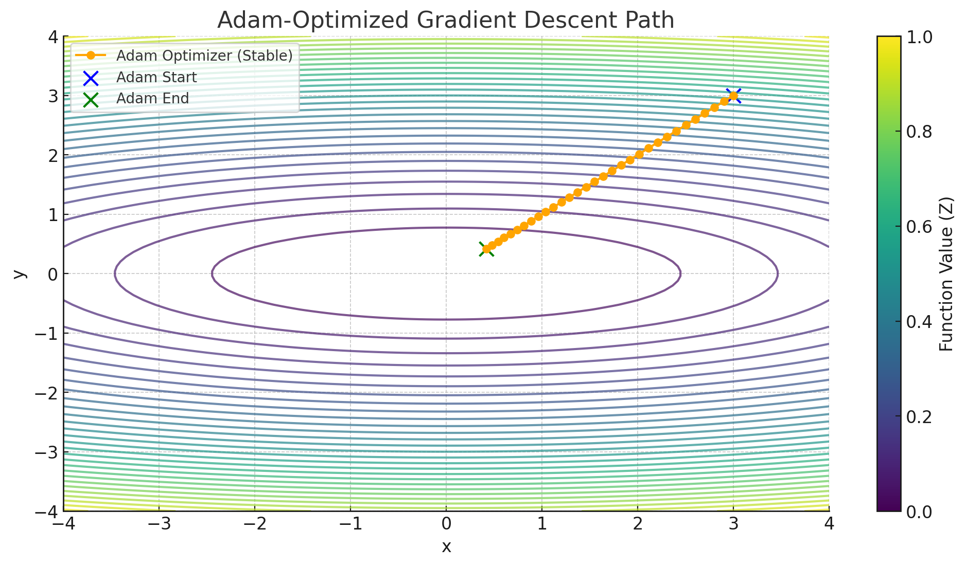
If you look at the next figure, you’ll see a scenario similar to the earlier demonstration of vanilla gradient descent, but this time the function is \(z = 0.1 x^2 + y^2\). We start at \((3, 3)\) and move toward the minimum at \((0, 0)\). Plain gradient descent can show noticeable oscillations when the curvature in the \(x\)-direction is different from the curvature in the \(y\)-direction. Adam, shown in the other figure, tends to navigate this terrain more smoothly, with fewer jolts or drastic overshoots. You can observe that its path is far less jittery, converging more directly toward the origin.
Adam is a powerful extension of gradient descent that incorporates both the momentum of past gradients and an adaptive scaling of updates. It often converges more quickly and is less sensitive to hyperparameter choices. Although no single optimization algorithm works perfectly for every problem, Adam has become a go-to method in many machine learning frameworks because it handles a wide range of tricky optimization challenges gracefully.